<?xml version="1.0" encoding="utf-8"?><feed xmlns="http://www.w3.org/2005/Atom" ><generator uri="https://jekyllrb.com/" version="3.10.0">Jekyll</generator><link href="https://vishalramesh.com/feed/foundational-ml.xml" rel="self" type="application/atom+xml" /><link href="https://vishalramesh.com/" rel="alternate" type="text/html" /><updated>2026-05-11T09:40:30+00:00</updated><id>https://vishalramesh.com/feed/foundational-ml.xml</id><title type="html">Vishal Ramesh | Foundationalml</title><subtitle>Vishal Ramesh - Machine Learning Engineer</subtitle><author><name>Vishal Ramesh</name></author><entry><title type="html">Gradient Descent</title><link href="https://vishalramesh.com/foundational-ml/optimizers/gradient-descent" rel="alternate" type="text/html" title="Gradient Descent" /><published></published><updated></updated><id>https://vishalramesh.com/foundational-ml/optimizers/gradient-descent</id><content type="html" xml:base="https://vishalramesh.com/foundational-ml/optimizers/gradient-descent"><![CDATA[<h2 id="gradient-descent">Gradient Descent</h2>

<p>Every function has <a href="https://vishalramesh.com/foundational-ml/math/notations-and-terminologies#maximas-and-minimas">minimas and maximas</a>. Gradient Descent is one way to find a minima.</p>

<p>Consider a function \(J(\theta)\). When we try to minimize it, we start at some randome \(\theta\), identify the <a href="https://vishalramesh.com/foundational-ml/math/differential-calculus#gradients">gradient</a> at that point, then update \(\theta\) by taking a step in the direction opposite to the gradient (with a controlled step size \(\alpha\)) to minimize \(J(\theta)\).</p>

<p><img src="https://vishalramesh.com/images/foundational-ml/optimizers/gradient-descent.png" alt="Gradient Descent" /></p>

<p>This is represented as
\(\theta_j := \theta_j - \alpha\frac{\delta}{\delta\theta_j}J(\theta)\)</p>

<p>Performing this opteration repeatedly, will bring us to a minima.</p>

<p>It is crucial to choose the right step size. Gradient descent with a low \(\alpha\) will take a long time to reach the minima, while a high \(\alpha\) might overshoot the minima.</p>

<p>When we process every sample in the training set to perform one step in the descent, it is called <strong>Batch Gradient Descent</strong>. This has one disadvantage. For large sets of data, the number of computations for every step or update is very large since we need to compute the gradient for the entire data set.</p>]]></content><author><name>Vishal Ramesh</name></author><category term="machine learning" /><category term="foundational-ml" /><category term="optimizers" /><summary type="html"><![CDATA[What is Gradient Descent?]]></summary></entry><entry><title type="html">Linear Models</title><link href="https://vishalramesh.com/foundational-ml/models/linear-models/" rel="alternate" type="text/html" title="Linear Models" /><published></published><updated></updated><id>https://vishalramesh.com/foundational-ml/models/linear-models</id><content type="html" xml:base="https://vishalramesh.com/foundational-ml/models/linear-models/"><![CDATA[<h2 id="linear-regression">Linear Regression</h2>
<p>
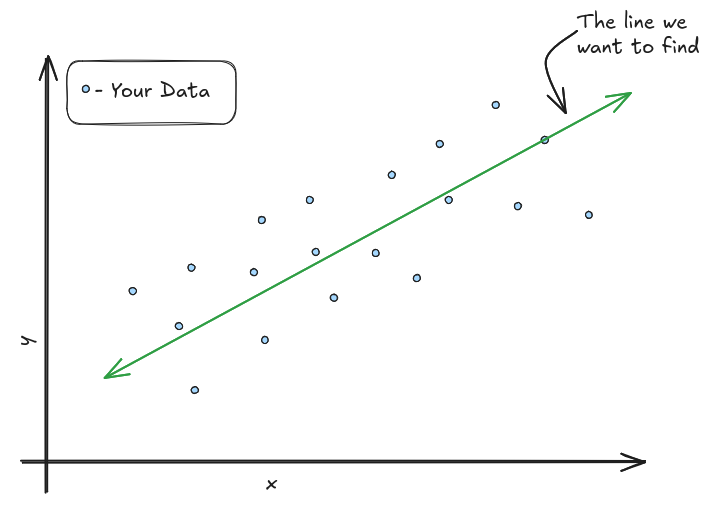
Linear Regression is a method used to model the relationship between a dependent variable and one or more independent variables by fitting a Linear Equation to the data. We basically try to find the best line (or plane or hyperplane depending on the dimensionality) that represents our data.</p>

<p><img src="https://vishalramesh.com/images/foundational-ml/linear-models/linear-regression.png" alt="Linear Regression" /></p>

<h2 id="how-does-it-work">How Does it Work?</h2>

<p>
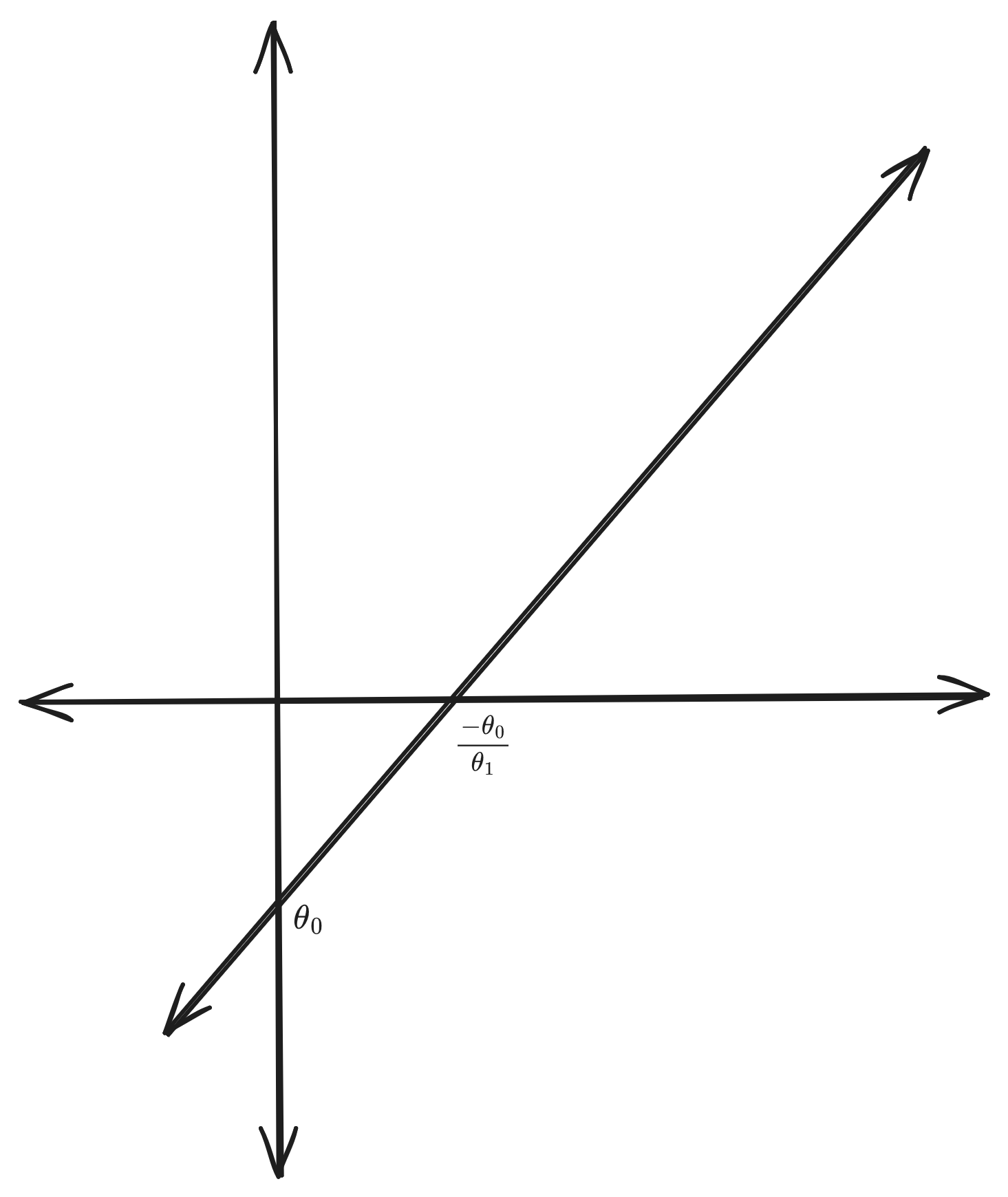
A linear equation with one independent variable (or feature) looks like this.
\(Y = \theta_0 + \theta_1\cdot X\)</p>

<p><img src="https://vishalramesh.com/images/foundational-ml/linear-models/mathematical-notation.png" alt="Mathematical Notation's Visualization" /></p>

<p>When you have more than one feature, it becomes</p>

\[Y = \theta_0 +\theta_1 \cdot X_1 + \theta_2 \cdot X_2 + ...\]

<p>which can be simplified into</p>

\[\sum_{j=0}^{n} \theta_j \cdot X_j\ \ \ \ \ \ where, X_0=1\\\]

<p>Also written as \(Y = h(X)\).</p>

<p>The above summation can be represented using matrices (for \(n=2\)) as</p>

\[\theta = \begin{matrix}
\theta_0 \\
\theta_1 \\
\theta_2 \\
\end{matrix}\ \ \ and\ \ \ X = \begin{matrix}
X_0 \\
X_1 \\
X_2 \\
\end{matrix}\]

<p>\(\theta\) is called the parameters (or weights) of the learning algorithm. The objective of the learning algorithm is to choose parameters \(\theta\) that allows us to make good predictions for \(Y\), i.e., Choose \(\theta\) such that \(h(x) \approx y\) for training samples.</p>

<p>To achieve this, we need to minimize the difference between \(h(x)\) and \(Y\) in the training samples. This difference is called the loss (or cost) and for linear regression, it is defined using the Mean Square Error (MSE). So our goal is to minimize the loss by adjusting \(\theta\).</p>

\[\underset{\theta}{minimize}\ \frac{1}{2}\sum_{i=1}^{m}J(\theta)\]

<p>where \(J(\theta) = (h_\theta(x^{(i)}) - y^{(i)})^2\), \(m\) is the number of training samples, and \(x^{(i)}\) and \(y^{(i)}\) are individual training samples.</p>

<p><em>The \(\frac{1}{2}\) is present just to make the gradient computation easier. When you differentiate the  squared component, the \(\frac{1}{2}\) will get cancelled in the result</em></p>

<h3 id="optimizing-using-gradient-descent">
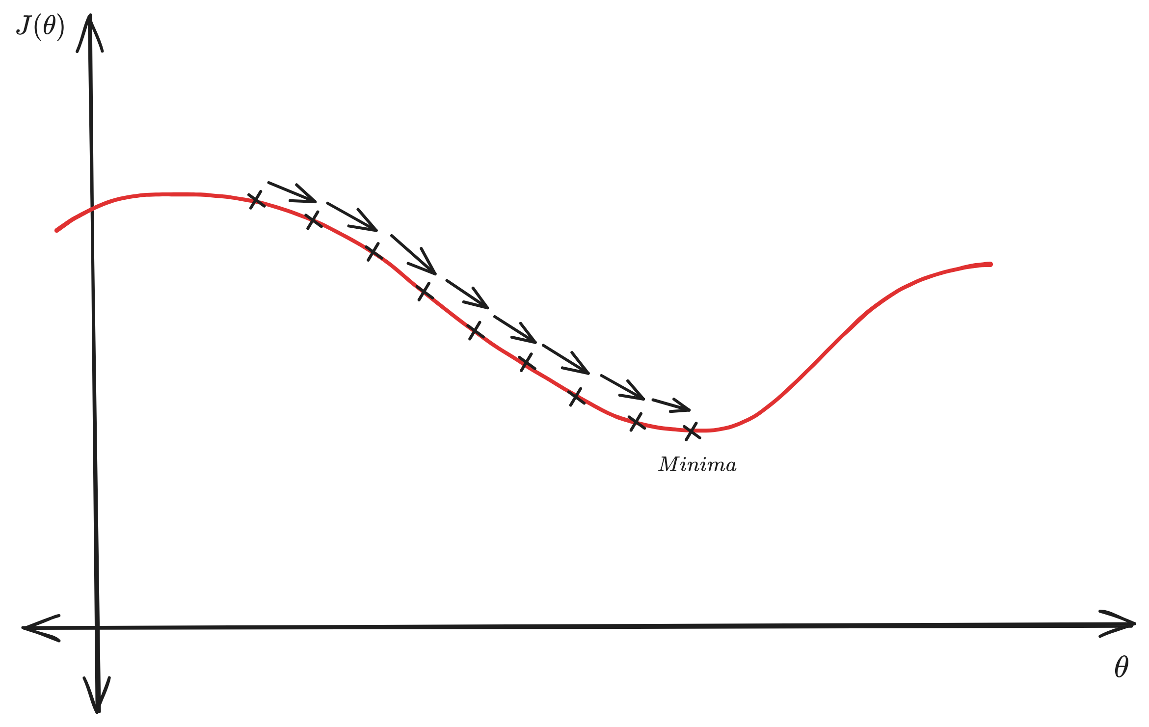
Optimizing using Gradient Descent</h3>
<p>There are a lot of optimizers that can be used to minimize the cost function. In this case, let&#8217;s look at <a href="https://vishalramesh.com/foundational-ml/optimizers/gradient-descent">Gradient Descent</a>.</p>

<p>For the cost function \(J(\theta)\) and model parameter \(\theta_j\), Gradient Descent is written as</p>

\[\theta_j := \theta_j - \alpha\frac{\delta}{\delta\theta_j}J(\theta)\]

<p>where \(\alpha\) is the learning rate.</p>

<p>So, continuing with the computation of the new value for \(\theta_j\),</p>

\[\frac{\delta}{\delta\theta_j} J(\theta) = \frac{\delta}{\delta\theta_j} \frac{1}{2}\sum_{i=1}^{m}(h_\theta(x^{(i)}) - y^{(i)})^2\]

<p>Ignoring the <a href="https://vishalramesh.com/foundational-ml/math/notations-and-terminologies#summation">\(\Sigma\)</a> and computing for a single training sample (for the sake of simplicity and the sum rule of differentiation),</p>

\[= \frac{\delta}{\delta\theta_j} \frac{1}{2}(h_\theta(x) - y)^2\]

\[= 2\cdot\frac{1}{2}(h_\theta(x)-y)\cdot\frac{\delta}{\delta\theta_j}(h_\theta(x)-y)\]

\[= (h_\theta(x)-y)\cdot\frac{\delta}{\delta\theta_j}(\theta_0x_0+\theta_1x_1...+\theta_nx_n-y)\]

<p>None of the terms inside the <a href="https://vishalramesh.com/foundational-ml/math/differential-calculus#partial-derivatives">partial derivative</a> depend on \(\theta_j\) except for \(\theta_jx_j\). So the partial derivative of all these terms are \(0\) and for \(\theta_jx_j\), it is \(x_j\). Therefore, the above expression simplifies into</p>

\[= (h_\theta(x)-y)\cdot x_j\]

<p>That gives us \(\theta_j := \theta_j - \alpha(h_\theta(x)-y)\cdot x_j\).</p>

<p>The above is for just one training sample. For the entire training set, we get</p>

\[\theta_j := \theta_j - \alpha\frac{1}{m}\sum_{i=1}^m(h_\theta(x^{(i)})-y^{(i)})\cdot x^{(i)}_j \ \ \ \ -\ Eq.\ 1\]

<p>and the derivative of the cost function when defined using all the training samples is</p>

\[\frac{\delta}{\delta\theta_j} J(\theta) = \sum_{i=1}^m(h_\theta(x^{(i)})-y^{(i)})\cdot x^{(i)}_j\]

<p>We&#8217;re including a \(\frac{1}{m}\) to avoid exploding gradients. When are add the gradients of all the training samples, the step size we take might increase with the size of the dataset. To avoid this, we&#8217;re averaging out the gradients using \(\frac{1}{m}\).</p>

<p>This is to optimize one parameter (which is used by one feature in the input matrix). So for a training sample with \(n\) features, Gradient descent becomes</p>
<div class="language-plaintext highlighter-rouge"><div class="highlight"><pre class="highlight"><code>for j = 0, 1, ..., n
  Eq. 1
</code></pre></div></div>

<p>This operation is also called <strong>Batch Gradient Descent</strong> because we process the entire dataset for every step in the descent.</p>

<p>Performing the Gradient Descent multiple times will eventually minimize the cost and give us a \(\theta\) that would be best fitting linear equation that models/describes the training data.</p>

<h2 id="additional-info">Additional Info</h2>
<ul>
  <li>The cost function (MSE) is a quadratic function. This means it has exactly one <a href="https://vishalramesh.com/foundational-ml/math/notations-and-terminologies#maximas-and-minimas">minima</a> (local and global minima are the same).</li>
  <li>For Linear Regression, you can find the optimal \(\theta\) (or global minima) in a single step using <a href="https://vishalramesh.com/foundational-ml/math/normal-equations">Normal Equations</a>.</li>
</ul>

<h2 id="simple-implementation-in-python">Simple Implementation in Python</h2>

<details>
  <summary><b>Show Code</b></summary>
<br />
  <script src="https://gist.github.com/fcb5eb918e1b49dfed7209167c06d14f.js?file=linear-regression.py"> </script>

</details>]]></content><author><name>Vishal Ramesh</name></author><category term="machine learning" /><category term="foundational-ml" /><category term="models" /><summary type="html"><![CDATA[Linear Models are one of the simplest Machine Learning algorithms. Let's look at how it works.]]></summary></entry><entry><title type="html">Some Math for Machine Learning</title><link href="https://vishalramesh.com/foundational-ml/math/" rel="alternate" type="text/html" title="Some Math for Machine Learning" /><published></published><updated></updated><id>https://vishalramesh.com/foundational-ml/some-math</id><content type="html" xml:base="https://vishalramesh.com/foundational-ml/math/"><![CDATA[<p><strong>NOTE</strong>: This is not a thorough coverage of all the math you&#8217;ll need for machine learning. This only includes concepts that will help better understand the algorithms and their mathematical breakdown covered in the <a href="https://vishalramesh.com/foundational-ml/">Foundational Machine Learning Series</a></p>

<ul>
  <li><a href="https://vishalramesh.com/foundational-ml/math/notations-and-terminologies">Mathematical Notations and Terminologies</a></li>
  <li><a href="https://vishalramesh.com/foundational-ml/math/matrix-multiplication">Matrix Multiplication</a></li>
  <li><a href="https://vishalramesh.com/foundational-ml/math/differential-calculus">Differential Calculus</a></li>
</ul>]]></content><author><name>Vishal Ramesh</name></author><category term="machine learning" /><category term="foundational-ml" /><category term="math" /><summary type="html"><![CDATA[Covers some math that will be useful to understand Machine Learning algorithms and its working]]></summary></entry><entry><title type="html">Mathematical Notations and Terminologies</title><link href="https://vishalramesh.com/foundational-ml/math/notations-and-terminologies" rel="alternate" type="text/html" title="Mathematical Notations and Terminologies" /><published></published><updated></updated><id>https://vishalramesh.com/foundational-ml/math/notations-and-terminologies</id><content type="html" xml:base="https://vishalramesh.com/foundational-ml/math/notations-and-terminologies"><![CDATA[<p>A lot of the notations and terminologies are explained using programming analogies wherever possible.</p>

<h2 id="summation">Summation</h2>

<p>Represented using \(\Sigma\), it is used to denote an iterative addition operation.</p>

<p>For example,
\(\sum_{i=0}^{n} x_i\)
is equivalent to</p>
<div class="language-python highlighter-rouge"><div class="highlight"><pre class="highlight"><code><span class="nb">sum</span> <span class="o">=</span> <span class="mi">0</span>
<span class="k">for</span> <span class="n">i</span> <span class="ow">in</span> <span class="nb">range</span><span class="p">(</span><span class="n">n</span><span class="p">):</span>
    <span class="nb">sum</span> <span class="o">+=</span> <span class="n">x</span><span class="p">[</span><span class="n">i</span><span class="p">]</span>
</code></pre></div></div>

<h2 id="derivative">Derivative</h2>

<p>Derivative or differentiation of a function \(f(x)\) w.r.t \(x\) is represented as \(\frac{d}{dx}f(x)\) or \(f'(x)\). For more info on derivates, check <a href="https://vishalramesh.com/foundational-ml/math/differential-calculus">here</a>.</p>

<h2 id="maximas-and-minimas">Maximas and Minimas</h2>
<p>In calculus, minima and maxima (collectively called extrema) are the &#8220;peaks&#8221; and &#8220;valleys&#8221; of a function.</p>
<ul>
  <li><strong>Local Extrema</strong>: These are the peaks or valleys within a specific neighborhood. A function can have many of these.</li>
  <li><strong>Global (Absolute) Extrema</strong>: These are the single highest or lowest points over the entire domain of the function.</li>
</ul>]]></content><author><name>Vishal Ramesh</name></author><category term="machine learning" /><category term="foundational-ml" /><category term="math" /><summary type="html"><![CDATA[Covers some mathematical notations and terminologies that will be useful to understand Machine Learning algorithms and its working.]]></summary></entry><entry><title type="html">Normal Equations</title><link href="https://vishalramesh.com/foundational-ml/math/normal-equations" rel="alternate" type="text/html" title="Normal Equations" /><published></published><updated></updated><id>https://vishalramesh.com/foundational-ml/math/normal-equations</id><content type="html" xml:base="https://vishalramesh.com/foundational-ml/math/normal-equations"><![CDATA[<p>Coming Soon&#8230;</p>]]></content><author><name>Vishal Ramesh</name></author><category term="machine learning" /><category term="foundational-ml" /><category term="math" /><summary type="html"><![CDATA[What are Normal Equations?]]></summary></entry><entry><title type="html">Matrix Multiplcation</title><link href="https://vishalramesh.com/foundational-ml/math/matrix-multiplication" rel="alternate" type="text/html" title="Matrix Multiplcation" /><published></published><updated></updated><id>https://vishalramesh.com/foundational-ml/math/matrix-multiplication</id><content type="html" xml:base="https://vishalramesh.com/foundational-ml/math/matrix-multiplication"><![CDATA[<h2 id="what-are-matrices">What are Matrices?</h2>

<p>Matrices are a rectangular arrangement of data. They can be numbers, variables, symbols or expressions. These are(https://vishalramesh.com/foundational-ml/math/notations-and-terminologies#maximas-and-minimas) represented in rows and columns.
Here&#8217;s an example:
\(numbers = \begin{bmatrix}
1 &amp; 4 &amp; 7 \\
2 &amp; 5 &amp; 8 \\
3 &amp; 6 &amp; 9
\end{bmatrix}\)
or
\(fruits = \begin{bmatrix}
banana &amp; apple &amp; mango \\
jackfruit &amp; tomato &amp; papaya \\
\end{bmatrix}\)</p>

<p>The shape of a matrix is represented as the (https://vishalramesh.com/foundational-ml/math/notations-and-terminologies#maximas-and-minimas)<code class="language-plaintext highlighter-rouge">number of rows X number of columns</code>. The shape of the matrix <code class="language-plaintext highlighter-rouge">numbers</code> is <code class="language-plaintext highlighter-rouge">3X3</code> and the shape of the matrix fruits is <code class="language-plaintext highlighter-rouge">2X3</code>.</p>

<h2 id="matrix-multiplication">Matrix Multiplication</h2>
<p>Consider two matrices
\(A = \begin{bmatrix}
a_{00} &amp; a_{01} &amp; a_{02} \\
a_{10} &amp; a_{11} &amp; a_{12} \\
a_{20} &amp; a_{21} &amp; a_{22}
\end{bmatrix}
,
B = \begin{bmatrix}
b_{00} &amp; b_{01} &amp; b_{02} \\
b_{10} &amp; b_{11} &amp; b_{12} \\
b_{20} &amp; b_{21} &amp; b_{22}
\end{bmatrix}\)</p>

<p>To multiply two matrices, you the the first row of the first matrix, and do a scalar multiplcation with the first column of the second matrix. This is the value of the first row&#8217;s first column. Repeat the process to build out the entire result matrix.</p>

<p>The product of these matrices \(A \cdot B\) or just \(AB\) is as follows.
\(B = \begin{bmatrix}
a_{00}b_{00} + a_{01}b_{10} + a_{02}b_{20} &amp; a_{00}b_{01} + a_{01}b_{11} + a_{02}b_{21} &amp; a_{00}b_{02} + a_{01}b_{12} + a_{02}b_{22} \\
a_{10}b_{00} + a_{11}b_{10} + a_{12}b_{20} &amp; a_{10}b_{01} + a_{11}b_{11} + a_{12}b_{21} &amp; a_{10}b_{02} + a_{11}b_{12} + a_{12}b_{22} \\
a_{20}b_{00} + a_{21}b_{10} + a_{22}b_{20} &amp; a_{20}b_{01} + a_{21}b_{11} + a_{22}b_{21} &amp; a_{20}b_{02} + a_{21}b_{12} + a_{22}b_{22} 
\end{bmatrix}\)</p>

<p>Check <a href="https://www.mathsisfun.com/algebra/matrix-multiplying.html">this</a> out if you want a more visual explanation or just scroll to the end of this page for a visualizer.</p>

<ul>
  <li>Matrix multiplication is not Commutative. So \(AB != BA\).</li>
  <li>To be able to multiply two matrices, the number of columns of the first matrix should be equal to the number of rows of the second matrix.</li>
</ul>

<h2 id="why-is-this-important-in-ml">Why is this important in ML?</h2>
<p>Machine Learning has a lot of linear algebra. We can represent these operations as matrices.</p>

<p>For example, consider the linear equation \(y = ax_{0} + bx_{1} + cx_{2}\). We can represent this using matrices as
\(y = \begin{bmatrix}
a &amp; b &amp; c
\end{bmatrix} \times \begin{bmatrix}
x_0\\
x_1\\
x_2
\end{bmatrix}\)
and there are a lot of matrix &#8220;features&#8221; that make solving linear equations much easier and faster. You&#8217;ll see them as you go.</p>

<p>Another advantage of using Matrices in machine learning is that it lets us speed up our processing. GPUs are really poweful at executing instructions in parallel that you can parallelize a large number of operations if you can represent them as matrix operations and perform them on a GPU.</p>

<div class="simd-visualizer" style="font-family: system-ui, sans-serif; max-width: 600px; margin: 0 auto; text-align: center; border: 1px solid #ddd; border-radius: 8px; padding: 20px; background: #fafafa; color: #222;">
  <h3 style="margin-top: 0; color: #222;">Matrix Multiplication: CPU vs GPU</h3>
  
  <div style="display: flex; justify-content: center; align-items: center; gap: 15px; margin-bottom: 20px;">
    <div id="matA" style="display: grid; grid-template-columns: repeat(3, 30px); gap: 5px;"></div>
    <div style="font-weight: bold; color: #555;">X</div>
    <div id="matB" style="display: grid; grid-template-columns: repeat(3, 30px); gap: 5px;"></div>
    <div style="font-weight: bold; color: #555;">=</div>
    <div id="matC" style="display: grid; grid-template-columns: repeat(3, 30px); gap: 5px;"></div>
  </div>

  <div style="display: flex; justify-content: center; gap: 10px;">
    <button onclick="runCPU()" style="padding: 10px 15px; border: none; background: #007bff; color: white; border-radius: 5px; cursor: pointer; font-weight: bold;">Compute Sequentially (CPU)</button>
    <button onclick="runGPU()" style="padding: 10px 15px; border: none; background: #28a745; color: white; border-radius: 5px; cursor: pointer; font-weight: bold;">Compute in Parallel (GPU)</button>
    <button onclick="resetVis()" style="padding: 10px 15px; border: 1px solid #ccc; background: #fff; border-radius: 5px; cursor: pointer; color: #222;">Reset</button>
  </div>

  <p id="vis-status" style="margin-top: 15px; font-weight: bold; min-height: 20px; color: #333;"></p>

  <style>
    .cell { width: 30px; height: 30px; display: flex; align-items: center; justify-content: center; background: #fff; border: 1px solid #ccc; border-radius: 4px; font-size: 14px; color: #222; transition: all 0.2s; }
    .cell.active-a { background: #ffeeba; border-color: #ffc107; transform: scale(1.1); z-index: 10;}
    .cell.active-b { background: #b8daff; border-color: #007bff; transform: scale(1.1); z-index: 10;}
    .cell.result-active { background: #c3e6cb; border-color: #28a745; font-weight: bold; color: #111; }
  </style>

  <script>
    const A = [[1, 2, 3], [4, 5, 6], [7, 8, 9]];
    const B = [[9, 8, 7], [6, 5, 4], [3, 2, 1]];
    let animationTimeout;

    function renderMatrix(id, data, empty = false) {
      const container = document.getElementById(id);
      if (!container) return;
      container.innerHTML = '';
      for (let i = 0; i < 3; i++) {
        for (let j = 0; j < 3; j++) {
          const cell = document.createElement('div');
          cell.className = 'cell';
          cell.id = `${id}-${i}-${j}`;
          cell.innerText = empty ? '' : data[i][j];
          container.appendChild(cell);
        }
      }
    }

    function resetVis() {
      clearTimeout(animationTimeout);
      renderMatrix('matA', A);
      renderMatrix('matB', B);
      renderMatrix('matC', [], true);
      const statusEl = document.getElementById('vis-status');
      if (statusEl) statusEl.innerText = 'Ready.';
    }

    function computeCell(r, c) {
      let sum = 0;
      for (let k = 0; k < 3; k++) sum += A[r][k] * B[k][c];
      return sum;
    }

    function clearHighlights() {
      document.querySelectorAll('.cell').forEach(el => el.classList.remove('active-a', 'active-b', 'result-active'));
    }

    function highlightRowCol(r, c) {
      clearHighlights();
      for(let k=0; k<3; k++) {
        const cellA = document.getElementById(`matA-${r}-${k}`);
        const cellB = document.getElementById(`matB-${k}-${c}`);
        if (cellA) cellA.classList.add('active-a');
        if (cellB) cellB.classList.add('active-b');
      }
    }

    function runCPU() {
      resetVis();
      document.getElementById('vis-status').innerText = 'Computing sequentially...';
      let r = 0, c = 0;

      function step() {
        if (r >= 3) {
          clearHighlights();
          document.getElementById('vis-status').innerText = 'Done! 9 iterations completed.';
          return;
        }
        highlightRowCol(r, c);
        const resCell = document.getElementById(`matC-${r}-${c}`);
        if (resCell) {
          resCell.innerText = computeCell(r, c);
          resCell.classList.add('result-active');
        }

        c++;
        if (c >= 3) { c = 0; r++; }
        animationTimeout = setTimeout(step, 600);
      }
      step();
    }

    function runGPU() {
      resetVis();
      document.getElementById('vis-status').innerText = 'Dispatching threads... Computing in parallel!';
      
      for(let i=0; i<3; i++) {
        for(let j=0; j<3; j++) {
          const cellA = document.getElementById(`matA-${i}-${j}`);
          const cellB = document.getElementById(`matB-${i}-${j}`);
          if (cellA) cellA.classList.add('active-a');
          if (cellB) cellB.classList.add('active-b');
        }
      }

      animationTimeout = setTimeout(() => {
        for(let r=0; r<3; r++) {
          for(let c=0; c<3; c++) {
            const resCell = document.getElementById(`matC-${r}-${c}`);
            if (resCell) {
              resCell.innerText = computeCell(r, c);
              resCell.classList.add('result-active');
            }
          }
        }
        document.getElementById('vis-status').innerText = 'Done! 1 step completed across 9 parallel threads.';
      }, 500); 
    }

    document.addEventListener('DOMContentLoaded', resetVis);
    // Fallback in case the script loads after DOM is ready
    if (document.readyState === "complete" || document.readyState === "interactive") {
        resetVis();
    }
  </script>
</div>

<p>There are more uses of matrices in machine learning. You&#8217;ll learn about them as you understand the algorithms and their implementations.</p>]]></content><author><name>Vishal Ramesh</name></author><category term="machine learning" /><category term="foundational-ml" /><category term="math" /><summary type="html"><![CDATA[What are Matrices? How do you Multiply them? Why do you need them in ML?]]></summary></entry><entry><title type="html">Differential Calculus</title><link href="https://vishalramesh.com/foundational-ml/math/differential-calculus" rel="alternate" type="text/html" title="Differential Calculus" /><published></published><updated></updated><id>https://vishalramesh.com/foundational-ml/math/differential-calculus</id><content type="html" xml:base="https://vishalramesh.com/foundational-ml/math/differential-calculus"><![CDATA[<p>Differential Calculus is a branch of calculus that deals with derivates, which is the rate of change of a function with respect to a variable.</p>

<h2 id="derivatives">Derivatives</h2>

<p>Lets look at an example. Consider an object travelling at a velocity w.r.t time defined by the function \(f(t)\). Meaning, at \(t=0\), the velocity is \(f(0)\), at \(t=1\), the velocity is \(f(1)\) and so on. For the sake of simplicity, let&#8217;s have \(f(t)\) be a linear function which will look something like this:</p>

<p>\(f(t) = a\cdot t + c\), where \(a\) and \(c\) are constants.
<img src="https://vishalramesh.com/images/foundational-ml/differential-calculus/linear-function.png" alt="Linear Velocity Function" /></p>

<p>The derivative in this case will tell us the variation in \(v\) for a unit \(t\) (for velocity, this is acceleration refers to). Basically, the derivative (\(\Delta\)) in this case would be \(f(t+1) - f(t)\). This when computed, will give us:
\(f(t+1) - f(t) = a\cdot(t+1) + c - (a\cdot t + c) \\
= a\cdot t + a + c - a\cdot t - c \\
= a\)</p>

<p>This was simple for a straight line where the rate of change stays the same. Now consider this curve:</p>

<p><img src="https://vishalramesh.com/images/foundational-ml/differential-calculus/non-linear-function.png" alt="Non -Linear Velocity Function" /></p>

<p>In the linear function, we could determine the derivative by just doing \(f(t+1) - f(t)\). But in the second, non-linear scenario, we can&#8217;t do that because the rate of change is also changing with time. Using the approach we used for the linear function would only give us the average rate of change for a unit time. It won&#8217;t work to find the rate of change at a specific point in time. 
So, instead of determining the change in a function (\(\Delta f\)) for a change in a variable (\(\Delta x\)), we try to identify the infinitesimally small change in the function (\(df(x)\)) for an infinitesimally small change in a variable (\(dx\)), i.e., \(\frac{df(x)}{fx}\).</p>

<p>A derivative of a function \(f(x)\) can be represented in several ways, some of them being \(f'(x)\), \(\frac{d}{dx}f(x)\) or \(\frac{df}{dx}\).</p>

<p>For some rules about computing derivates and derivatives of some common functions, check <a href="https://www.mathsisfun.com/calculus/derivatives-rules.html">here</a>.</p>

<h2 id="partial-derivatives">Partial Derivatives</h2>

<p>In the above section we saw an example where we had a function that had only one variable. Now, consider a function that has multiple variables \(f(x,y,z,...)\).</p>

<p>Partial derivates tell us how a function like this changes while tweaking only one variable, but keeping the rest as constant.</p>

<p>Partial derivative of \(f\) w.r.t \(x\) is represented as \(\frac{\delta f}{\delta x}\).</p>

<p>Computing the a partial derivative follows the same rules as a regular derivate, you just treat all the variables w.r.t which you&#8217;re computing the gradient as constants. So in the above function \(f(x,y,z...)\), for \(\frac{\delta f}{\delta x}\), you&#8217;ll treat \(x\) as the only variable.</p>

<h2 id="gradients">Why is this useful?</h2>

<p>Gradients are a large part of training machine learning algorithms and optimization functions. A gradient of the function \(f\) is just a bundle of all the partial derivatives of the function.
\(\nabla f = \begin{bmatrix}
\frac{\delta f}{\delta x}, \frac{\delta f}{\delta y}, \frac{\delta f}{\delta z}, ...
\end{bmatrix}\)</p>

<p>The gradient acts as a compass which always points in the direction of the steepest ascent.</p>]]></content><author><name>Vishal Ramesh</name></author><category term="machine learning" /><category term="foundational-ml" /><category term="math" /><summary type="html"><![CDATA[What is differential calculus?]]></summary></entry></feed>