Differential Calculus

Differential Calculus is a branch of calculus that deals with derivates, which is the rate of change of a function with respect to a variable.

Derivatives

Lets look at an example. Consider an object travelling at a velocity w.r.t time defined by the function \(f(t)\). Meaning, at \(t=0\), the velocity is \(f(0)\), at \(t=1\), the velocity is \(f(1)\) and so on. For the sake of simplicity, let’s have \(f(t)\) be a linear function which will look something like this:

\(f(t) = a\cdot t + c\), where \(a\) and \(c\) are constants.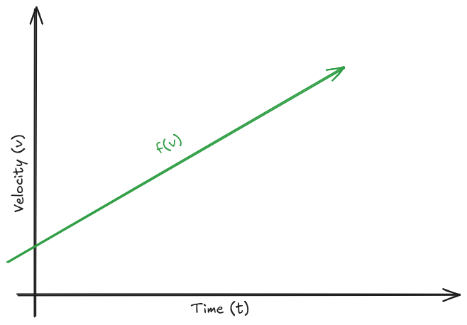

The derivative in this case will tell us the variation in \(v\) for a unit \(t\) (for velocity, this is acceleration refers to). Basically, the derivative (\(\Delta\)) in this case would be \(f(t+1) - f(t)\). This when computed, will give us: \(f(t+1) - f(t) = a\cdot(t+1) + c - (a\cdot t + c) \\ = a\cdot t + a + c - a\cdot t - c \\ = a\)

This was simple for a straight line where the rate of change stays the same. Now consider this curve:

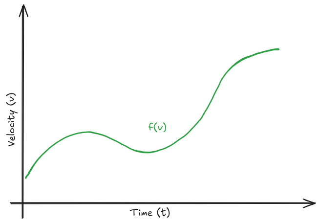
In the linear function, we could determine the derivative by just doing \(f(t+1) - f(t)\). But in the second, non-linear scenario, we can’t do that because the rate of change is also changing with time. Using the approach we used for the linear function would only give us the average rate of change for a unit time. It won’t work to find the rate of change at a specific point in time. So, instead of determining the change in a function (\(\Delta f\)) for a change in a variable (\(\Delta x\)), we try to identify the infinitesimally small change in the function (\(df(x)\)) for an infinitesimally small change in a variable (\(dx\)), i.e., \(\frac{df(x)}{fx}\).

A derivative of a function \(f(x)\) can be represented in several ways, some of them being \(f'(x)\), \(\frac{d}{dx}f(x)\) or \(\frac{df}{dx}\).

For some rules about computing derivates and derivatives of some common functions, check here.

Partial Derivatives

In the above section we saw an example where we had a function that had only one variable. Now, consider a function that has multiple variables \(f(x,y,z,...)\).

Partial derivates tell us how a function like this changes while tweaking only one variable, but keeping the rest as constant.

Partial derivative of \(f\) w.r.t \(x\) is represented as \(\frac{\delta f}{\delta x}\).

Computing the a partial derivative follows the same rules as a regular derivate, you just treat all the variables w.r.t which you’re computing the gradient as constants. So in the above function \(f(x,y,z...)\), for \(\frac{\delta f}{\delta x}\), you’ll treat \(x\) as the only variable.

Why is this useful?

Gradients are a large part of training machine learning algorithms and optimization functions. A gradient of the function \(f\) is just a bundle of all the partial derivatives of the function. \(\nabla f = \begin{bmatrix} \frac{\delta f}{\delta x}, \frac{\delta f}{\delta y}, \frac{\delta f}{\delta z}, ... \end{bmatrix}\)

The gradient acts as a compass which always points in the direction of the steepest ascent.