Gradient Descent

Gradient Descent

Every function has minimas and maximas. Gradient Descent is one way to find a minima.

Consider a function \(J(\theta)\). When we try to minimize it, we start at some randome \(\theta\), identify the gradient at that point, then update \(\theta\) by taking a step in the direction opposite to the gradient (with a controlled step size \(\alpha\)) to minimize \(J(\theta)\).

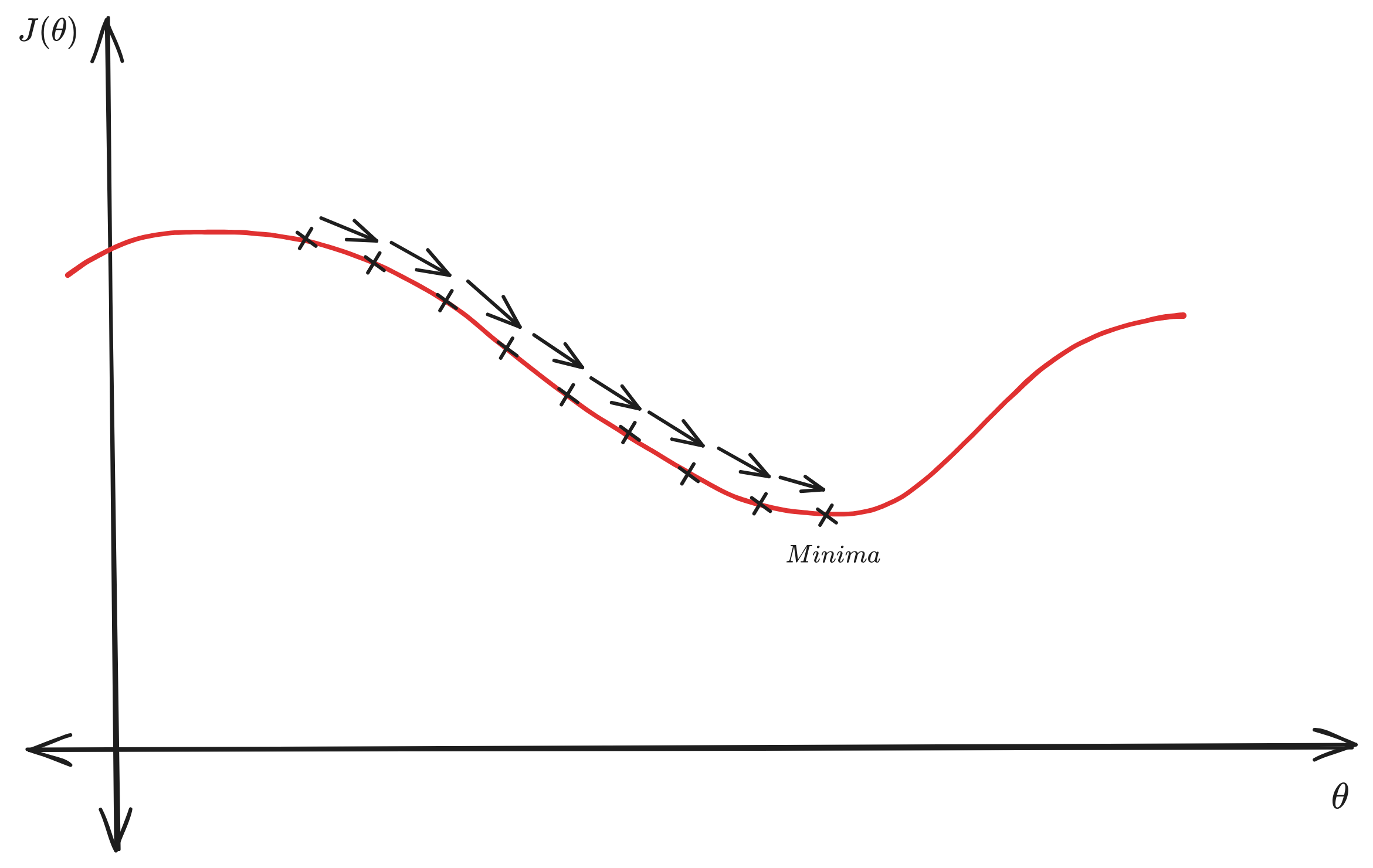
This is represented as \(\theta_j := \theta_j - \alpha\frac{\delta}{\delta\theta_j}J(\theta)\)

Performing this opteration repeatedly, will bring us to a minima.

It is crucial to choose the right step size. Gradient descent with a low \(\alpha\) will take a long time to reach the minima, while a high \(\alpha\) might overshoot the minima.

When we process every sample in the training set to perform one step in the descent, it is called Batch Gradient Descent. This has one disadvantage. For large sets of data, the number of computations for every step or update is very large since we need to compute the gradient for the entire data set.